Copy raster values in vector fields then read vector

This example shows how to extract from polygons or points each pixel centroid located in the vector (polygons/points) and how to extract and save band values in vector fields.

This tool is made to avoid using raster everytime you need to learn and predict a model.

Import librairies

import museotoolbox as mtb
from matplotlib import pyplot as plt

Load HistoricalMap dataset

raster,vector = mtb.datasets.load_historical_data(low_res=True)
out_vector='/tmp/vector_withROI.gpkg'

Note

There is no need to specify a bandPrefix. If bandPrefix is not specified, scipt will only generate the centroid

mtb.processing.sample_extraction(raster,vector,
                                 out_vector=out_vector,
                                 unique_fid='uniquefid',
                                 band_prefix='band_',
                                 verbose=False)

Read values from both vectors

originalY = mtb.processing.read_vector_values(vector,'Class')
X,y = mtb.processing.read_vector_values(out_vector,'Class',band_prefix='band_')

Original vector is polygon type, each polygons contains multiple pixel

print(originalY.shape)

Out:

(17,)

Number of Y in the new vector is the total number of pixel in the polygons

print(y.shape)

Out:

(3175,)

X has the same size of Y, but in 3 dimensions because our raster has 3 bands

print(X.shape)
print(X[410:420,:])
print(y[410:420])

Out:

(3175, 3)
[[209 184 153]
 [ 81 109 114]
 [122 142 147]
 [145 160 161]
 [135 130  89]
 [109 108  75]
 [109 108  75]
 [119 102  85]
 [126 131  91]
 [122 110  88]]
[3 4 4 4 1 1 1 1 1 1]

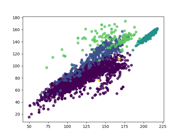
Plot blue and red band

plt.figure(1)
colors =  [int(i % 23) for i in y]
plt.scatter(X[:,0],X[:,2],c=colors,alpha=.8)
plt.show()