Learn with Random-Forest and Random Sampling 50% (RS50)

This example shows how to make a Random Sampling with 50% for each class.

Import librairies

from museotoolbox.ai import SuperLearner
from museotoolbox.cross_validation import RandomStratifiedKFold
from museotoolbox.processing import extract_ROI
from museotoolbox import datasets
from sklearn.ensemble import RandomForestClassifier
from sklearn import metrics

Load HistoricalMap dataset

raster,vector = datasets.load_historical_data(low_res=True)
field = 'Class'
X,y = extract_ROI(raster,vector,field)

Create CV

SKF = RandomStratifiedKFold(n_splits=2,
                random_state=12,verbose=False)

Initialize Random-Forest and metrics

classifier = RandomForestClassifier(random_state=12,n_jobs=1)

#
kappa = metrics.make_scorer(metrics.cohen_kappa_score)
f1_mean = metrics.make_scorer(metrics.f1_score,average='micro')
scoring = dict(kappa=kappa,f1_mean=f1_mean,accuracy='accuracy')

Start learning

sklearn will compute different metrics, but will keep best results from kappa (refit=’kappa’)

SL = SuperLearner(classifier=classifier,param_grid = dict(n_estimators=[10]),n_jobs=1,verbose=1)

SL.fit(X,y,cv=SKF,scoring=kappa)


# =============================================================================
# ##############################################################################
# # Read the model
# # -------------------
# print(SL.model)
# print(SL.model.cv_results_)
# print(SL.model.best_score_)
#
# ##############################################################################
# # Get F1 for every class from best params
# # -----------------------------------------------
#
# for stats in SL.get_stats_from_cv(confusion_matrix=False,F1=True):
#     print(stats['F1'])
#
# ##############################################################################
# # Get each confusion matrix from folds
# # -----------------------------------------------
#
# for stats in SL.get_stats_from_cv(confusion_matrix=True):
#     print(stats['confusion_matrix'])
#
# ##############################################################################
# # Save each confusion matrix from folds
# # -----------------------------------------------
#
# SL.save_cm_from_cv('/tmp/testMTB/',prefix='RS50_')
#
# =============================================================================

Out:

Fitting 2 folds for each of 1 candidates, totalling 2 fits
[Parallel(n_jobs=1)]: Using backend SequentialBackend with 1 concurrent workers.
[Parallel(n_jobs=1)]: Done   2 out of   2 | elapsed:    0.1s finished
best score : 0.9098953680202182
best n_estimators : 10

Predict map

SL.predict_image(raster,'/tmp/classification.tif',
                  higher_confidence='/tmp/confidence.tif',
                  confidence_per_class='/tmp/confidencePerClass.tif')

Out:

Total number of blocks : 6
Detected 1 band for function predict_array.
No data is set to : 0.
Detected 5 bands for function predict_confidence_per_class.
No data is set to : -32768.
Detected 1 band for function predict_higher_confidence.
No data is set to : -32768.
Batch processing (6 blocks using 23Mo of ram)

Prediction... [##......................................]5%

Prediction... [####....................................]11%

Prediction... [######..................................]16%

Prediction... [########................................]22%

Prediction... [###########.............................]27%

Prediction... [#############...........................]33%

Prediction... [###############.........................]38%

Prediction... [#################.......................]44%

Prediction... [####################....................]50%

Prediction... [######################..................]55%

Prediction... [########################................]61%

Prediction... [##########################..............]66%

Prediction... [############################............]72%

Prediction... [###############################.........]77%

Prediction... [#################################.......]83%

Prediction... [###################################.....]88%

Prediction... [#####################################...]94%

Prediction... [#######################################.]99%

Prediction... [########################################]100%

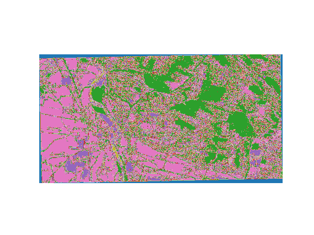
Plot example

from matplotlib import pyplot as plt
from osgeo import gdal
src=gdal.Open('/tmp/classification.tif')
plt.imshow(src.GetRasterBand(1).ReadAsArray(),cmap=plt.get_cmap('tab20'))
plt.axis('off')
plt.show()