Note
Click here to download the full example code
Learn algorithm and customize your input raster without writing it on disk
This example shows how to customize your raster (ndvi, smooth signal…) in the learning process to avoi generate a new raster.
Import librairies
from museotoolbox.ai import SuperLearner
from museotoolbox.processing import extract_ROI
from museotoolbox import datasets
from sklearn.ensemble import RandomForestClassifier
from sklearn import metrics
Load HistoricalMap dataset
raster,vector = datasets.load_historical_data(low_res=True)
field = 'Class'
Initialize Random-Forest and metrics
classifier = RandomForestClassifier(random_state=12,n_jobs=1)

kappa = metrics.make_scorer(metrics.cohen_kappa_score)
f1_mean = metrics.make_scorer(metrics.f1_score,average='micro')
scoring = dict(kappa=kappa,f1_mean=f1_mean,accuracy='accuracy')
Start learning
sklearn will compute different metrics, but will keep best results from kappa (refit=’kappa’)
SL = SuperLearner(classifier=classifier,param_grid=dict(n_estimators=[10]),n_jobs=1,verbose=1)
Create or use custom function
def reduceBands(X,bandToKeep=[0,2]):
    # this function get the first and the last band
    X=X[:,bandToKeep].reshape(-1,len(bandToKeep))
    return X

# add this function to learnAndPredict class
SL.customize_array(reduceBands)

# if you learn from vector, refit according to the f1_mean
X,y = extract_ROI(raster,vector,field)
SL.fit(X,y,cv=2,scoring=scoring,refit='f1_mean')
Out:
Fitting 2 folds for each of 1 candidates, totalling 2 fits
[Parallel(n_jobs=1)]: Using backend SequentialBackend with 1 concurrent workers.
[Parallel(n_jobs=1)]: Done   2 out of   2 | elapsed:    0.1s finished
best score : 0.9135528815706142
best n_estimators : 10
Read the model
print(SL.model)
print(SL.model.cv_results_)
print(SL.model.best_score_)
Out:
GridSearchCV(cv=<museotoolbox.cross_validation.RandomStratifiedKFold object at 0x7ff586391a50>,
             error_score=nan,
             estimator=RandomForestClassifier(bootstrap=True, ccp_alpha=0.0,
                                              class_weight=None,
                                              criterion='gini', max_depth=None,
                                              max_features='auto',
                                              max_leaf_nodes=None,
                                              max_samples=None,
                                              min_impurity_decrease=0.0,
                                              min_impurity_split=None,
                                              min_samples_leaf=1,
                                              min_...
                                              min_weight_fraction_leaf=0.0,
                                              n_estimators=100, n_jobs=1,
                                              oob_score=False, random_state=12,
                                              verbose=0, warm_start=False),
             iid='deprecated', n_jobs=1, param_grid={'n_estimators': [10]},
             pre_dispatch='2*n_jobs', refit='f1_mean', return_train_score=False,
             scoring={'accuracy': 'accuracy',
                      'f1_mean': make_scorer(f1_score, average=micro),
                      'kappa': make_scorer(cohen_kappa_score)},
             verbose=1)
{'mean_fit_time': array([0.01987207]), 'std_fit_time': array([0.00012457]), 'mean_score_time': array([0.00556481]), 'std_score_time': array([0.00013554]), 'param_n_estimators': masked_array(data=[10],
             mask=[False],
       fill_value='?',
            dtype=object), 'params': [{'n_estimators': 10}], 'split0_test_kappa': array([0.84275596]), 'split1_test_kappa': array([0.85203727]), 'mean_test_kappa': array([0.84739662]), 'std_test_kappa': array([0.00464065]), 'rank_test_kappa': array([1], dtype=int32), 'split0_test_f1_mean': array([0.91070298]), 'split1_test_f1_mean': array([0.91640279]), 'mean_test_f1_mean': array([0.91355288]), 'std_test_f1_mean': array([0.00284991]), 'rank_test_f1_mean': array([1], dtype=int32), 'split0_test_accuracy': array([0.91070298]), 'split1_test_accuracy': array([0.91640279]), 'mean_test_accuracy': array([0.91355288]), 'std_test_accuracy': array([0.00284991]), 'rank_test_accuracy': array([1], dtype=int32)}
0.9135528815706142
Get F1 for every class from best params
for stats in SL.get_stats_from_cv(confusion_matrix=False,F1=True):
    print(stats['F1'])
Out:
[Parallel(n_jobs=1)]: Using backend SequentialBackend with 1 concurrent workers.
[Parallel(n_jobs=1)]: Done   2 out of   2 | elapsed:    0.0s finished
[0.94209703 0.74862385 0.99824253 0.752      0.        ]
[0.94649351 0.7678245  0.99647887 0.74137931 0.        ]
Get each confusion matrix from folds
for stats in SL.get_stats_from_cv(confusion_matrix=True):
    print(stats['confusion_matrix'])
Out:
[Parallel(n_jobs=1)]: Using backend SequentialBackend with 1 concurrent workers.
[Parallel(n_jobs=1)]: Done   2 out of   2 | elapsed:    0.0s finished
[[903  38   0   1   0]
 [ 71 204   0  11   0]
 [  0   0 284   0   0]
 [  0  17   1  47   1]
 [  1   0   0   0   0]]
[[911  30   0   0   1]
 [ 70 210   0   6   0]
 [  0   0 283   1   0]
 [  1  21   1  43   0]
 [  1   0   0   0   0]]
Save each confusion matrix from folds
SL.save_cm_from_cv('/tmp/testMTB/',prefix='RS50_')
Out:
[Parallel(n_jobs=1)]: Using backend SequentialBackend with 1 concurrent workers.
[Parallel(n_jobs=1)]: Done   1 out of   1 | elapsed:    0.0s remaining:    0.0s
[Parallel(n_jobs=1)]: Done   2 out of   2 | elapsed:    0.1s finished
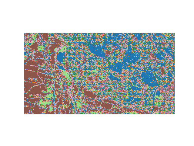
Predict map
SL.predict_image(raster,'/tmp/classification.tif',
                  higher_confidence='/tmp/confidence.tif',
                  confidence_per_class='/tmp/confidencePerClass.tif')
Out:
Total number of blocks : 6
Detected 1 band for function predict_array.
Detected 5 bands for function predict_confidence_per_class.
Detected 1 band for function predict_higher_confidence.
Batch processing (6 blocks using 23Mo of ram)

Prediction... [##......................................]5%

Prediction... [####....................................]11%

Prediction... [######..................................]16%

Prediction... [########................................]22%

Prediction... [###########.............................]27%

Prediction... [#############...........................]33%

Prediction... [###############.........................]38%

Prediction... [#################.......................]44%

Prediction... [####################....................]50%

Prediction... [######################..................]55%

Prediction... [########################................]61%

Prediction... [##########################..............]66%

Prediction... [############################............]72%

Prediction... [###############################.........]77%

Prediction... [#################################.......]83%

Prediction... [###################################.....]88%

Prediction... [#####################################...]94%

Prediction... [#######################################.]99%

Prediction... [########################################]100%
Plot example
from matplotlib import pyplot as plt
from osgeo import gdal
src=gdal.Open('/tmp/classification.tif')
plt.imshow(src.GetRasterBand(1).ReadAsArray(),cmap=plt.get_cmap('tab20'))
plt.axis('off')
plt.show()
Total running time of the script: ( 0 minutes 1.124 seconds)