Compute Moran’s I with different lags from raster

Compute Moran’s I with different lags, support mask.

Import librairies

import numpy as np
from museotoolbox.stats import Moran
from matplotlib import pyplot as plt
from osgeo import gdal,osr

Load HistoricalMap dataset

raster = '/tmp/autocorrelated_moran.tif'
mask = '/tmp/mask.tif'

def create_false_image(array,path):
    # from https://pcjericks.github.io/py-gdalogr-cookbook/raster_layers.html
    driver = gdal.GetDriverByName('GTiff')
    outRaster = driver.Create(path, array.shape[1], array.shape[0], 1, gdal.GDT_Byte)
    outRaster.SetGeoTransform((0, 10, 0, 0, 0, 10))
    outband = outRaster.GetRasterBand(1)
    outband.WriteArray(array)
    outRasterSRS = osr.SpatialReference()
    outRasterSRS.ImportFromEPSG(4326)
    outRaster.SetProjection(outRasterSRS.ExportToWkt())
    outband.FlushCache()

# create autocorrelated tif
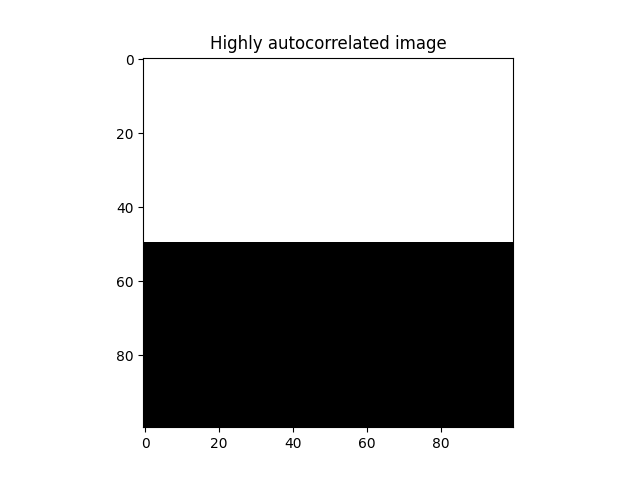
x = np.zeros((100,100),dtype=int)
# max autocorr
x[:50,:] = 1
create_false_image(x,raster)
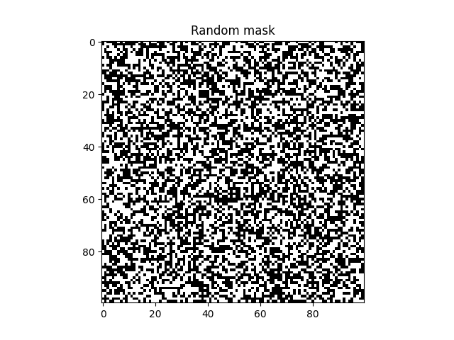
x_mask = np.random.randint(0,2,[100,100])
create_false_image(x_mask,mask)

Random mask

plt.title('Random mask')
plt.imshow(x_mask,cmap='gray', aspect='equal',interpolation='none')

Out:

<matplotlib.image.AxesImage object at 0x7f7fdd636210>

Spatially autocorrelated image

plt.title('Highly autocorrelated image')
plt.imshow(x,cmap='gray', aspect='equal',interpolation='none')

Out:

<matplotlib.image.AxesImage object at 0x7f7fdf88e910>

Compute Moran’s I for lag 1 on autocorrelated image

lags =  [1,3,5]

MoransI = Moran(raster,lag=lags,in_image_mask=mask)
print(MoransI.scores)

Out:

{'lag': [1, 3, 5], 'I': [0.985906052599945, 0.9650410397190331, 0.9452969276242092], 'band': [1, 1, 1], 'EI': [-0.00019968051118210862, -0.00019968051118210862, -0.00019968051118210862]}

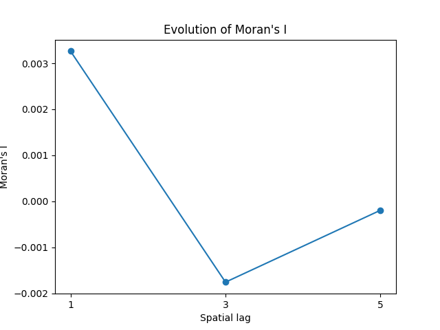
Compute Moran’s I for lag 1 on totally random image

lags =  [1,3,5]

MoransI = Moran(mask,lag=lags)
print(MoransI.scores)

Out:

{'lag': [1, 3, 5], 'I': [0.0032631012391146704, -0.0017543519080462694, -0.0001922459568890084], 'band': [1, 1, 1], 'EI': [-0.00010001000100010001, -0.00010001000100010001, -0.00010001000100010001]}

Plot result

from matplotlib import pyplot as plt
plt.title('Evolution of Moran\'s I')
plt.plot(MoransI.scores['lag'],MoransI.scores['I'],'-o')
plt.xlabel('Spatial lag')
plt.xticks(lags)
plt.ylabel('Moran\'s I')

Out:

Text(0, 0.5, "Moran's I")